
Motivation
In the past we often were faced with inadequate data. We had to rely on various hand-computed models and estimate using statistical tables. In the modern world, we have quite the opposite problem. Now we have too much data. With this much data, it is very inefficient, or even dangerous, to consider all data as being equally useful. Our problem then is how do we find out the most relevant features of the data.
Prerequisites of this guide:
- An understanding of eigenvectors and eigendecomposition of matrices is essential to understand this guide.
What Principle Component Analysis does
As I’ve said, our problem is to distill the many features down to just the most important ones. This improves our computation efficiency and removes a lot of the noise. This process is known as dimensionality reduction. Throughout this guide, we’ll start by having 2 dimensions (features). Our job will be to combine/remove one of them to find a single most important feature. We can then generalize this to finding the k most important features.
Structure of the guide:
Since this is a very comprehensive guide, we’ll go step-by-step:
- What dimensionality reduction means
- Understanding the relationship between data and and ellipses
- Understanding the quadratic form of an ellipse
- Understanding the eigendecomposition of an ellipse
- Understanding the relation between the symmetric matrix of an ellipse and the covariance matrix of data
- Performing the eigenvector decomposition of the covariance matrix of the data to find the principal components
- Picking the k largest eigenvalues and their related eigenvectors
- Projecting the entire data/ellipse using the basis formed by the eigenvectors to find the k most important features
Dimensionality Reduction
Suppose I have a dataset with two numerical features. I plot a scatter plot. In it, the green data point represents one class and the red data point represents another. My job is to create a model that uses the two features to predict the class of the data point.
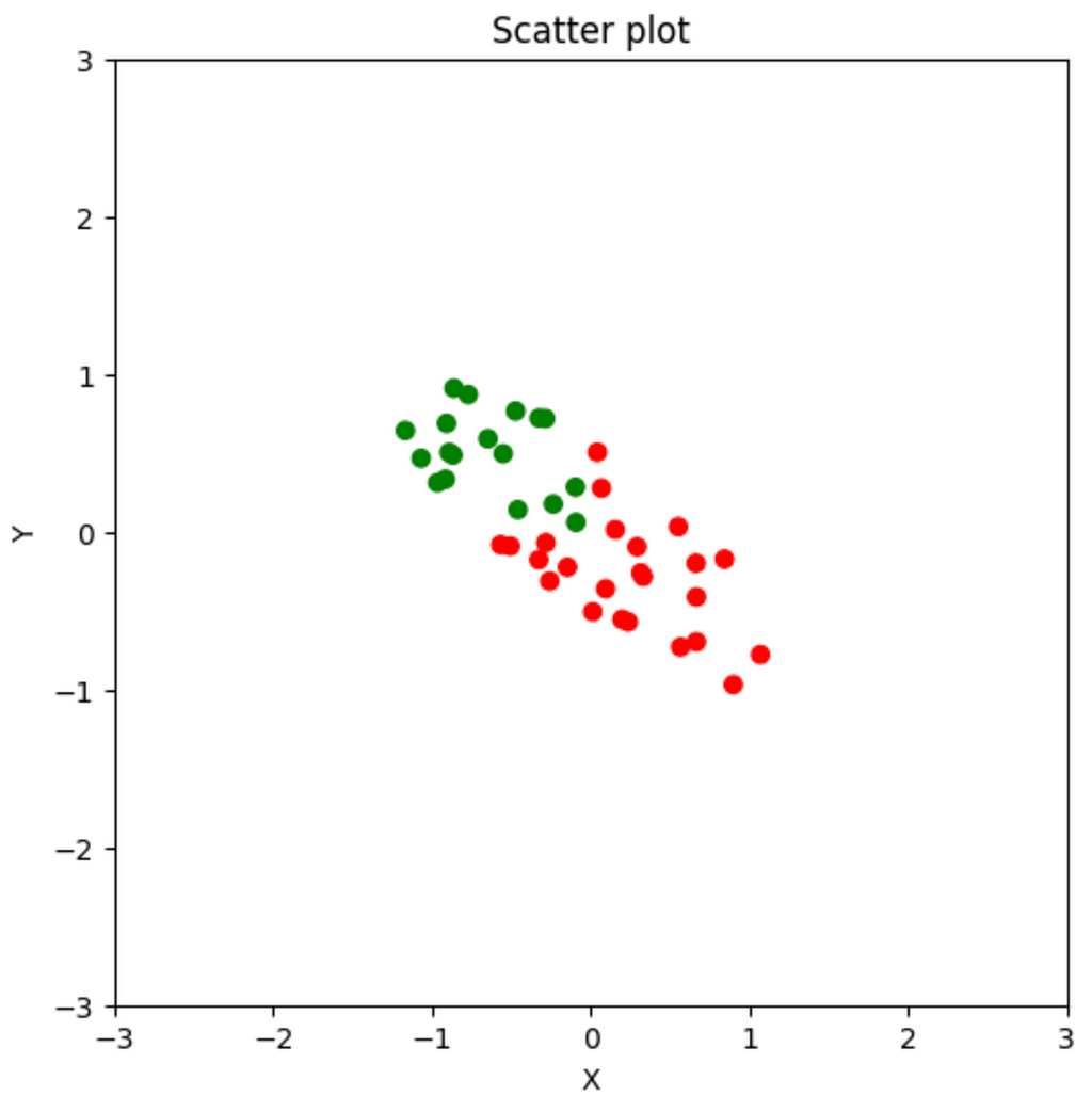
My goal is to find a single feature that best represents the data. The idea here is to find a direction of movement that best describes the variability of the data. This is the features that best describes the data (Why?). Then we can ignore everything else. This will be the same as somehow projecting all the data points on a single number line. Then we can have a single threshold. The data points to the left of that threshold are green and the data points to the right are red. This greatly simplifies the computation that our algorithm needs to do. You can imagine that if we’re able to condense 5000 features into 50, how much more efficient that would be.
To understand how we do this, we’ll have to go through some theory.
Ellipses
Standard Ellipses
We begin our study of PCA with ellipses. An ellipses is a stretched out circle. A standard ellipse (no rotation and centered about the origin) has the cartesian equation:


Some terminology about ellipses:
- c represents the focal points of the ellipse and can be found through a and b. We won’t worry about that in this guide.
- The major axis of the ellipse is the direction of the most stretch. In this case it is the x-axis
- The minor axis of the ellipse is perpendicular to the major axis. In this case it is the y-axis
Non-standard ellipse
We will consider ellipses which are centered about the origin and have some non-zero rotation (If our ellipse isn’t centered about the origin, we can simply subtract the center of the ellipse from each point and we’ll get a centered ellipse). Such an ellipse is represented by the quadratic form:

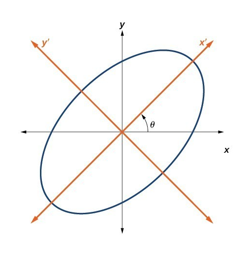
Such an ellipse is difficult to work with. The semi axes (major and minor) are at an angle so we will need to account for rotation in every calculation we do. It would be a much more easier if we take x' and y' as our axes. In that case the entire ellipse will look like any normal ellipse. If the ellipse represented our data points, you can see why the entire dataset will be easier to interpret if it was standard. The problem of eigendecomposition attempts to solve this problem in this context.
Note: The quadratic form also represents hyperbolas, but we’re only considering the values of a, b, and c such that the resulting figure is an ellipse
Relationship between data and ellipses
For every numerical dataset, we can draw an ellipse around every point. Since we’re dealing with 2d right now, we’ll draw a 2d ellipse around our data points:
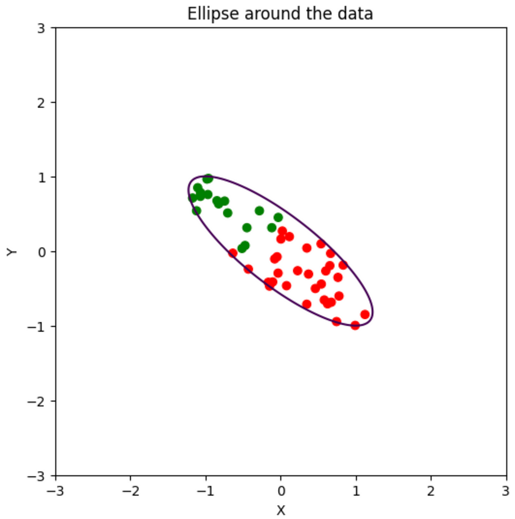
Notice the following: The biggest spread in the data is from top-left to bottom-right. Also, the major axis of the ellipse around the data is also in the same direction. So, if we wanna find the direction of maximum variation, we better find the direction of this axis. The minor axis of this ellipse represents the next best direction. Since our data only has 2 features, the maximum number of features we can extract is 2. If we have to only pick 1 feature, the feature in the direction of the major axis is our best bet. From intuition it appears to be a linear combination of some positive x feature and some negative y feature. Let’s see how we can do that
The symmetric matrix of the quadratic form
Consider the quadratic form of the non-standard ellipse:
Let’s encode the same equation in terms of matrices
Let X be the coordinate vector:

Let A be the coefficient matrix:

I picked that peculiar matrix because now, the entire quadratic form can be expressed as the matrix equation:

I highly recommend you simplify this matrix equation to see that it is indeed the quadratic form of the ellipse.
Important note: The diagonal of the symmetric matrix represents the coefficient of the quadratic terms. The off-diagonal coefficients represent the mixed terms
Eigendecomposition refresher (Standardizing the ellipse)
Our steps are actually very easy:
- If our ellipse isn’t centered around (0, 0), then subtract the ellipse’s center (mean), to center it
- Find the eigenvectors of the symmetric matrix (They represent the directions of the major and minor axes)
- Project the entire ellipse using the matrix formed by the eigenvectors
Suppose that our ellipse is already centered around the origin. We find the matrices P and D such that

Since A is a symmetric matrix, the spectral theorem states that P is also orthogonal. So its inverse is its transpose


Where Y represents a new coordinate system found by projecting the x and y basis through the eigenvectors.
Why does Y give the direction of the major and minor axes of the ellipse?
Consider the equation of the unit circle:

Think of A as a transformation matrix from this unit circle to an ellipse. The eigenvectors of this matrix represent those vectors who do not get thrown off their span. For a standard ellipse, A is a diagonal matrix, so its eigenvectors are normal basis vectors. Also the axes of the ellipse are along these same directions. So eigenvectors of the symmetric matrix for an ellipse provide the direction of the major and minor axes. It shouldn’t be too difficult to think of why this is true for a non-standard matrix too.
The Covariance Matrix
In practice, we don’t need to use ellipses everytime we want to find the features that represent the most variability. We use the covariance matrix. The covariance matrix for 2 features is the following matrix:

The diagonal represents the variances of each feature. Everything else is the covariance of each feature with every other feature. It is an alternative to the symmetric matrix we used for the ellipse. The entire matrix represents the variability of the data in each direction.
Relation between the covariance and the symmetric matrix
Here is my claim: The information stored in the covariance matrix is the same that is stored in the symmetric matrix. And here is why:
- The eigenvectors of the covariance matrix represent the directions of maximum variability. The eigenvectors of the symmetric matrix represent the directions of the semi-axes (major, minor) of the ellipse. Since the most variability should be about the major axes, the directions of the eigenvectors of both the matrices should be the same
- The eigenvalues of the covariance matrix represent the variability along the eigenvectors. The eigenvalues of the symmetric matrix are the inverse square-roots of the lengths of the major and minor axes. So the eigenvalues must be completely different
So, for our data set, it should be the same if we calculate the eigenstuff of the covariance matrix or the symmetric matrix. Let’s test that hypothesis out:
The equation of the ellipse that I’m using is:

So, its symmetric matrix must be:

Similarly, using Python, I’ve calculated the covariance matrix:

The matrices are nothing alike, but let’s perform the eigendecomposition of the matrices:
Symmetric matrix:
np.linalg.eig(sym_matrix)- Eigenvalues: 0.43844719, 4.56155281
- Eigenvectors=[-0.78820544, 0.61541221], [ -0.61541221, -0.78820544]
Covariance matrix:
np.linalg.eig(df.cov())- Eigenvalues: 0.8381163 , 0.13917908
- Eigenvectors=[ 0.79329999, -0.60883096], [0.60883096, 0.79329999]
The eigenvalues are completely different for the matrices, but the eigenvectors are almost the same. This is because the points are randomly plotted within the ellipse and do not perfectly represent the ellipse.
Since the eigenvalues of the symmetric matrix are inversely proportional to the square-root length of the axes, the major axis of the ellipse must be in the direction of the second eigenvector (Calculate them and check). Since the eigenvalues of the covariance matrix represent the variability along the direction of the eigenvector, the major axis of the data-points must be the first eigenvector. Look at that! Both the matrices agree.
Using the eigenvectors: Projection
Finally, since we have the eigenvectors, we can find the principle component (Features with the maximum variability). We are reducing our dimension from 2 to 1. So we only get to pick 1 feature. In this case, it will be our first eigenvector. So our feature is:

Now, how do we use this? This equation came from the eigenvector with the biggest eigenvalue. We will dot the eigenvector with every point in our dataset. This will result in a 1-d line which looks like:
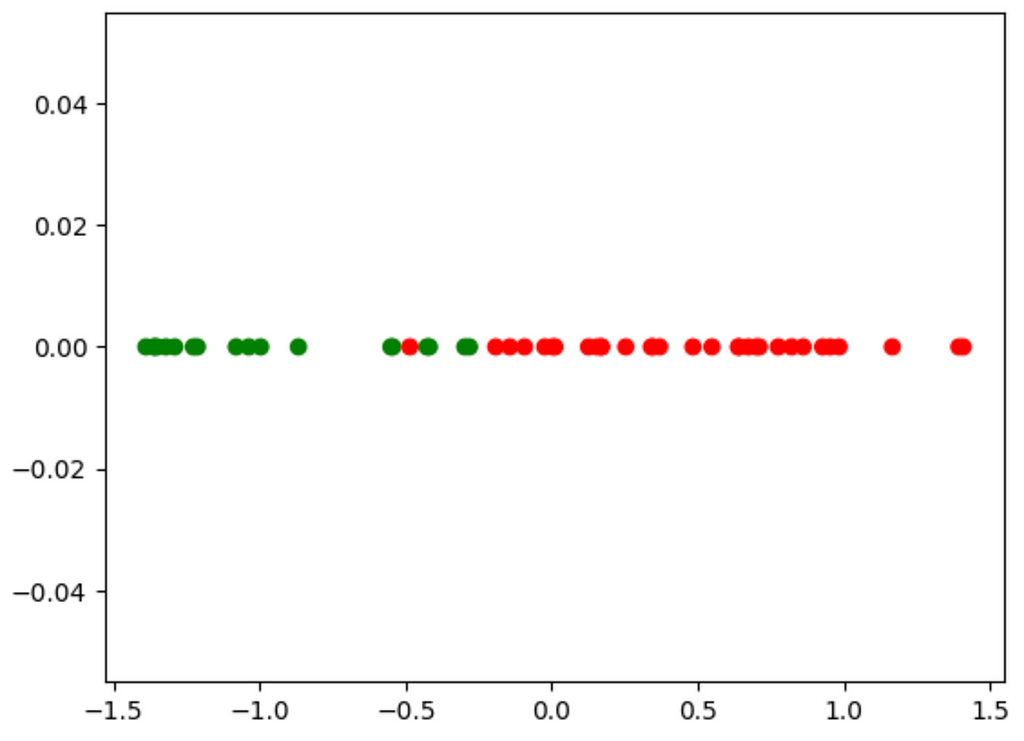
Though we have lost some information by ignoring the other eigenvector, we have retained the most important information. From this, we can create a very simple model to classify the points. Eye-balling it, it looks like about -0.25 is the threshold, though there is one red outlier in the greens. We don’t even need a complex ML model to classify these data points.
For every new data point we get, we will calculate this new feature using the equation, check if its below -0.25, then classify it accordingly.
Summary of the process
All in all, here is the process of PCA:
- Standardize the data
- Find covariance/correlation matrix
- Find eigenstuff of the matrix
- Pick the k largest eigenvalues
- Make a projection matrix of the eigenvectors of those eigenvalues
- Transform the entire data using the projection matrix
Now, as code:
# The data points
df = pd.DataFrame({'x': x_coords, 'y': y_coords})
# Eigendecomposition
eig_vals, eig_vecs = np.linalg.eig(df.cov())
eig_pairs = [(np.abs(eig_vals[i]), eig_vecs[:,i]) for i in range(len(eig_vals))]
# Sorting eig_pairs by the eigenvalue
eig_pairs.sort(key=lambda x: x[0], reverse=True)
# Picking the k best eigenvectors (k = 1)
k = 1
projection_matrix = np.hstack([eig_pairs[i][1].reshape(-1, 1) for i in range(k)])
# Projecting the points and plotting the new x values
projected_points = np.array(df[['x', 'y']]).dot(projection_matrix)
# Plotting the projected points
plt.scatter(projected_points[:, 0], [0]*len(projected_points[:, 0]), color=colors)
plt.show()Or, using sklearn:
from sklearn.decompose import PCA

pca = PCA(n_components = 1)
results = pca.fit_transform(df[["x", "y"]])
plt.scatter(results[:, 0], [0]*len(results[:, 0]), color=colors)
Conclusion
In this blog, we’ve explored the motivation and fundamental concepts behind Principal Component Analysis (PCA). We began by addressing the challenge of handling excessive data and the necessity of identifying the most relevant features for improved computational efficiency. We delved into the basics of dimensionality reduction, using ellipses to understand data variability and the role of eigenvectors and eigendecomposition. Finally, we demonstrated how to project data onto principal components, highlighting the practical implementation in Python. Thank you for reading this guide!